Autores: Davi Toshio e Henrique Cursino Vieira

Carregando as bibliotecas
library(dplyr)
library(ggplot2)
library(tidyr)
library(readr)
library(caret)
library(ranger)
library(rpart)
library(rpart.plot)
library(corrplot)
library(statisticalModeling)
library(mlbench)
library(e1071)
Este kernel é uma aplicação prática de análise exploratória de dados e aprendizado de máquina utilizando a linguagem R. Aqui analisamos os dados do desafio “House Prices: Advanced Regression /Techniques”, do repositório Kaggle.
Link: https://www.kaggle.com/c/house-prices-advanced-regression-techniques
1.Pré-tratamento dos dados
1.2.Carregando teste e treino
setwd('/home/davi/Desktop/house_prices-_advanced_regression_techniques/')

train <- read.csv(file = 'train.csv', sep= ',', stringsAsFactors = F)
test <- read.csv(file = 'test.csv', sep= ',', stringsAsFactors = F)

# Adicionando coluna SalePrice no conjunto teste
test$SalePrice <- NA

# Criando coluna index do data set
train$dataset <- 'train'
test$dataset <- 'test'

# Juntando dataset, melhora
joined_data <- rbind(train, test)
1.3.Definição de tipos e eliminação de variáveis
# Remove coluna Utilities (super representatividade de um fator)
which(colnames(joined_data) == 'Utilities')
## [1] 10joined_data <- joined_data[ ,-10]
# Outlier data$GarageYrBlt 2207 to 2007
joined_data$GarageYrBlt[which(joined_data$GarageYrBlt == 2207)] <- 2007
# Ajustando conteudo de variáveis onde NA é um factor
joined_data$Alley[which(is.na(joined_data$Alley))] <- 'no_alley_access'
joined_data$BsmtQual[which(is.na(joined_data$BsmtQual))] <- 'no_basement'
joined_data$BsmtCond[which(is.na(joined_data$BsmtCond))] <- 'no_basement'
joined_data$BsmtFinType1[which(is.na(joined_data$BsmtFinType1))] <- 'no_basement'
joined_data$BsmtFinType2[which(is.na(joined_data$BsmtFinType2))] <- 'no_basement'
joined_data$PoolQC[which(is.na(joined_data$PoolQC))] <- 'no_pool'
joined_data$Fence[which(is.na(joined_data$Fence))] <- 'no_fence'
joined_data$MiscFeature[which(is.na(joined_data$MiscFeature))] <- 'none'
joined_data$BsmtExposure[which(is.na(joined_data$BsmtExposure))] <- 'no_basemente'
joined_data$FireplaceQu[which(is.na(joined_data$FireplaceQu))] <- 'no_fireplace'
joined_data$GarageType[which(is.na(joined_data$GarageType))] <- 'no_garage'
joined_data$GarageFinish[which(is.na(joined_data$GarageFinish))] <- 'no_garage'
joined_data$GarageQual[which(is.na(joined_data$GarageQual))] <- 'no_garage'
joined_data$GarageCond[which(is.na(joined_data$GarageCond))] <- 'no_garage'
# Definindo e convertendo as variaveis categoricas (factors)
joined_data$MSSubClass <- as.factor(joined_data$MSSubClass)
joined_data$OverallQual <- as.factor(joined_data$OverallQual)
joined_data$OverallCond <- as.factor(joined_data$OverallCond)
joined_data$GarageYrBlt <- as.factor(joined_data$GarageYrBlt)
joined_data$YrSold <- as.factor(joined_data$YrSold)
joined_data$MoSold <- as.factor(joined_data$MoSold)
joined_data$GarageYrBlt <- as.factor(joined_data$GarageYrBlt)
joined_data$YearBuilt <- as.factor(joined_data$YearBuilt)
joined_data$YearRemodAdd <- as.factor(joined_data$YearRemodAdd)
# Coverte caracteres para factors
joined_data[ ,which(sapply(joined_data, is.character))] <- lapply(joined_data[ ,which(sapply(joined_data, is.character))], as.factor)
# BsmtFinSF1
na_position <- which(is.na(joined_data$BsmtFinSF1))
# Via de regra, para todo no_basement nas variaveis Bsmt, o valor e zero!
joined_data %>% select(contains('Bsmt')) %>%
filter( BsmtFinType1== 'no_basement') %>%
summary()## BsmtQual BsmtCond BsmtExposure BsmtFinType1
## Ex : 0 Fa : 0 Av : 0 ALQ : 0
## Fa : 0 Gd : 0 Gd : 0 BLQ : 0
## Gd : 0 no_basement:79 Mn : 0 GLQ : 0
## no_basement:79 Po : 0 No : 0 LwQ : 0
## TA : 0 TA : 0 no_basemente:79 no_basement:79
## Rec : 0
## Unf : 0
## BsmtFinSF1 BsmtFinType2 BsmtFinSF2 BsmtUnfSF TotalBsmtSF
## Min. :0 ALQ : 0 Min. :0 Min. :0 Min. :0
## 1st Qu.:0 BLQ : 0 1st Qu.:0 1st Qu.:0 1st Qu.:0
## Median :0 GLQ : 0 Median :0 Median :0 Median :0
## Mean :0 LwQ : 0 Mean :0 Mean :0 Mean :0
## 3rd Qu.:0 no_basement:79 3rd Qu.:0 3rd Qu.:0 3rd Qu.:0
## Max. :0 Rec : 0 Max. :0 Max. :0 Max. :0
## NA's :1 Unf : 0 NA's :1 NA's :1 NA's :1
## BsmtFullBath BsmtHalfBath
## Min. :0 Min. :0
## 1st Qu.:0 1st Qu.:0
## Median :0 Median :0
## Mean :0 Mean :0
## 3rd Qu.:0 3rd Qu.:0
## Max. :0 Max. :0
## NA's :2 NA's :2# BsmtFinSF1
joined_data$BsmtFinSF1[which(is.na(joined_data$BsmtFinSF1))] <- 0
# BsmtFinSF2
joined_data$BsmtFinSF2[which(is.na(joined_data$BsmtFinSF2))] <- 0
# BsmtUnfSF
joined_data$BsmtUnfSF[which(is.na(joined_data$BsmtUnfSF))] <- 0
# TotalBsmtSF
joined_data$TotalBsmtSF[which(is.na(joined_data$TotalBsmtSF))] <- 0
# BsmtFullBath
joined_data$BsmtFullBath[which(is.na(joined_data$BsmtFullBath))] <- 0
# BsmtHalfBath
joined_data$BsmtHalfBath[which(is.na(joined_data$BsmtHalfBath))] <- 0
# GarageCars
# Igual ao problema anterior, vemos que nas demais variaveis relacionada
# Temos 'no_garage', logo podemos colocar zero quando nao existir informacao
joined_data$GarageCars[which(is.na(joined_data$GarageCars))] <- 0
# GarageArea
joined_data$GarageArea[which(is.na(joined_data$GarageArea))] <- 0
# GarageYrBlt
# Variavel troll: onde tem NA, esta relacionado com no_garage ... --'
joined_data$GarageYrBlt <- as.character(joined_data$GarageYrBlt)
joined_data$GarageYrBlt[which(is.na(joined_data$GarageYrBlt))] <- 'no_garage'
joined_data$GarageYrBlt <- as.factor(joined_data$GarageYrBlt)
# Separa coluna de factors para analisar
col_factor <- which(sapply(joined_data, is.factor))
joined_data_factors <- joined_data[ , col_factor]
# Separa coluna de numericos
col_numeric <- which(sapply(joined_data, is.numeric))
names(joined_data[,col_numeric])## [1] "Id" "LotFrontage" "LotArea" "MasVnrArea"
## [5] "BsmtFinSF1" "BsmtFinSF2" "BsmtUnfSF" "TotalBsmtSF"
## [9] "X1stFlrSF" "X2ndFlrSF" "LowQualFinSF" "GrLivArea"
## [13] "BsmtFullBath" "BsmtHalfBath" "FullBath" "HalfBath"
## [17] "BedroomAbvGr" "KitchenAbvGr" "TotRmsAbvGrd" "Fireplaces"
## [21] "GarageCars" "GarageArea" "WoodDeckSF" "OpenPorchSF"
## [25] "EnclosedPorch" "X3SsnPorch" "ScreenPorch" "PoolArea"
## [29] "MiscVal" "SalePrice"1.4.Distribuição dos factors nas variável categóricas
Uma quantidade significativa das variáveis categóricas estão bem desproporcionais … :( Este é um problema que precisa ser melhor trabalhado futuramente. Elas são informativas, porém podem causar problema em nosso modelo.
# Coluna SalePrice: 32
list_of_var_counts <- apply(joined_data_factors, 2, function(x){

    table <- data.frame(table(x), as.numeric(table(x)/sum(table(x))))
    colnames(table) <- c('factor_type', 'raw_count', 'percentage')
    return(table)

})
list_of_var_counts
## $MSSubClass
## factor_type raw_count percentage
## 1 120 182 0.0623501199
## 2 150 1 0.0003425831
## 3 160 128 0.0438506338
## 4 180 17 0.0058239123
## 5 190 61 0.0208975677
## 6 20 1079 0.3696471394
## 7 30 139 0.0476190476
## 8 40 6 0.0020554985
## 9 45 18 0.0061664954
## 10 50 287 0.0983213429
## 11 60 575 0.1969852689
## 12 70 128 0.0438506338
## 13 75 23 0.0078794108
## 14 80 118 0.0404248030
## 15 85 48 0.0164439877
## 16 90 109 0.0373415553
##
## $MSZoning
## factor_type raw_count percentage
## 1 C (all) 25 0.008576329
## 2 FV 139 0.047684391
## 3 RH 26 0.008919383
## 4 RL 2265 0.777015437
## 5 RM 460 0.157804460
##
## $Street
## factor_type raw_count percentage
## 1 Grvl 12 0.004110997
## 2 Pave 2907 0.995889003
##
## $Alley
## factor_type raw_count percentage
## 1 Grvl 120 0.04110997
## 2 no_alley_access 2721 0.93216855
## 3 Pave 78 0.02672148
##
## $LotShape
## factor_type raw_count percentage
## 1 IR1 968 0.331620418
## 2 IR2 76 0.026036314
## 3 IR3 16 0.005481329
## 4 Reg 1859 0.636861939
##
## $LandContour
## factor_type raw_count percentage
## 1 Bnk 117 0.04008222
## 2 HLS 120 0.04110997
## 3 Low 60 0.02055498
## 4 Lvl 2622 0.89825283
##
## $LotConfig
## factor_type raw_count percentage
## 1 Corner 511 0.175059952
## 2 CulDSac 176 0.060294621
## 3 FR2 85 0.029119561
## 4 FR3 14 0.004796163
## 5 Inside 2133 0.730729702
##
## $LandSlope
## factor_type raw_count percentage
## 1 Gtl 2778 0.951695786
## 2 Mod 125 0.042822885
## 3 Sev 16 0.005481329
##
## $Neighborhood
## factor_type raw_count percentage
## 1 Blmngtn 28 0.009592326
## 2 Blueste 10 0.003425831
## 3 BrDale 30 0.010277492
## 4 BrkSide 108 0.036998972
## 5 ClearCr 44 0.015073655
## 6 CollgCr 267 0.091469681
## 7 Crawfor 103 0.035286057
## 8 Edwards 194 0.066461117
## 9 Gilbert 165 0.056526208
## 10 IDOTRR 93 0.031860226
## 11 MeadowV 37 0.012675574
## 12 Mitchel 114 0.039054471
## 13 NAmes 443 0.151764303
## 14 NoRidge 71 0.024323398
## 15 NPkVill 23 0.007879411
## 16 NridgHt 166 0.056868791
## 17 NWAmes 131 0.044878383
## 18 OldTown 239 0.081877355
## 19 Sawyer 151 0.051730045
## 20 SawyerW 125 0.042822885
## 21 Somerst 182 0.062350120
## 22 StoneBr 51 0.017471737
## 23 SWISU 48 0.016443988
## 24 Timber 72 0.024665982
## 25 Veenker 24 0.008221994
##
## $Condition1
## factor_type raw_count percentage
## 1 Artery 92 0.031517643
## 2 Feedr 164 0.056183625
## 3 Norm 2511 0.860226105
## 4 PosA 20 0.006851662
## 5 PosN 39 0.013360740
## 6 RRAe 28 0.009592326
## 7 RRAn 50 0.017129154
## 8 RRNe 6 0.002055498
## 9 RRNn 9 0.003083248
##
## $Condition2
## factor_type raw_count percentage
## 1 Artery 5 0.0017129154
## 2 Feedr 13 0.0044535800
## 3 Norm 2889 0.9897225077
## 4 PosA 4 0.0013703323
## 5 PosN 4 0.0013703323
## 6 RRAe 1 0.0003425831
## 7 RRAn 1 0.0003425831
## 8 RRNn 2 0.0006851662
##
## $BldgType
## factor_type raw_count percentage
## 1 1Fam 2425 0.83076396
## 2 2fmCon 62 0.02124015
## 3 Duplex 109 0.03734156
## 4 Twnhs 96 0.03288798
## 5 TwnhsE 227 0.07776636
##
## $HouseStyle
## factor_type raw_count percentage
## 1 1.5Fin 314 0.107571086
## 2 1.5Unf 19 0.006509078
## 3 1Story 1471 0.503939705
## 4 2.5Fin 8 0.002740665
## 5 2.5Unf 24 0.008221994
## 6 2Story 872 0.298732443
## 7 SFoyer 83 0.028434395
## 8 SLvl 128 0.043850634
##
## $OverallQual
## factor_type raw_count percentage
## 1 1 4 0.001370332
## 2 10 31 0.010620075
## 3 2 13 0.004453580
## 4 3 40 0.013703323
## 5 4 226 0.077423775
## 6 5 825 0.282631038
## 7 6 731 0.250428229
## 8 7 600 0.205549846
## 9 8 342 0.117163412
## 10 9 107 0.036656389
##
## $OverallCond
## factor_type raw_count percentage
## 1 1 7 0.002398082
## 2 2 10 0.003425831
## 3 3 50 0.017129154
## 4 4 101 0.034600891
## 5 5 1645 0.563549161
## 6 6 531 0.181911614
## 7 7 390 0.133607400
## 8 8 144 0.049331963
## 9 9 41 0.014045906
##
## $YearBuilt
## factor_type raw_count percentage
## 1 1872 1 0.0003425831
## 2 1875 1 0.0003425831
## 3 1879 1 0.0003425831
## 4 1880 5 0.0017129154
## 5 1882 1 0.0003425831
## 6 1885 2 0.0006851662
## 7 1890 7 0.0023980815
## 8 1892 2 0.0006851662
## 9 1893 1 0.0003425831
## 10 1895 3 0.0010277492
## 11 1896 1 0.0003425831
## 12 1898 1 0.0003425831
## 13 1900 29 0.0099349092
## 14 1901 2 0.0006851662
## 15 1902 1 0.0003425831
## 16 1904 1 0.0003425831
## 17 1905 3 0.0010277492
## 18 1906 1 0.0003425831
## 19 1907 1 0.0003425831
## 20 1908 2 0.0006851662
## 21 1910 43 0.0147310723
## 22 1911 1 0.0003425831
## 23 1912 5 0.0017129154
## 24 1913 1 0.0003425831
## 25 1914 8 0.0027406646
## 26 1915 24 0.0082219938
## 27 1916 10 0.0034258308
## 28 1917 3 0.0010277492
## 29 1918 10 0.0034258308
## 30 1919 5 0.0017129154
## 31 1920 57 0.0195272354
## 32 1921 11 0.0037684138
## 33 1922 16 0.0054813292
## 34 1923 17 0.0058239123
## 35 1924 16 0.0054813292
## 36 1925 34 0.0116478246
## 37 1926 19 0.0065090785
## 38 1927 9 0.0030832477
## 39 1928 9 0.0030832477
## 40 1929 8 0.0027406646
## 41 1930 26 0.0089071600
## 42 1931 7 0.0023980815
## 43 1932 5 0.0017129154
## 44 1934 5 0.0017129154
## 45 1935 13 0.0044535800
## 46 1936 11 0.0037684138
## 47 1937 9 0.0030832477
## 48 1938 13 0.0044535800
## 49 1939 20 0.0068516615
## 50 1940 36 0.0123329908
## 51 1941 23 0.0078794108
## 52 1942 6 0.0020554985
## 53 1945 15 0.0051387461
## 54 1946 15 0.0051387461
## 55 1947 11 0.0037684138
## 56 1948 27 0.0092497431
## 57 1949 18 0.0061664954
## 58 1950 38 0.0130181569
## 59 1951 18 0.0061664954
## 60 1952 18 0.0061664954
## 61 1953 24 0.0082219938
## 62 1954 43 0.0147310723
## 63 1955 34 0.0116478246
## 64 1956 39 0.0133607400
## 65 1957 35 0.0119904077
## 66 1958 48 0.0164439877
## 67 1959 43 0.0147310723
## 68 1960 37 0.0126755738
## 69 1961 34 0.0116478246
## 70 1962 35 0.0119904077
## 71 1963 35 0.0119904077
## 72 1964 33 0.0113052415
## 73 1965 34 0.0116478246
## 74 1966 35 0.0119904077
## 75 1967 41 0.0140459061
## 76 1968 45 0.0154162384
## 77 1969 28 0.0095923261
## 78 1970 42 0.0143884892
## 79 1971 39 0.0133607400
## 80 1972 40 0.0137033231
## 81 1973 21 0.0071942446
## 82 1974 23 0.0078794108
## 83 1975 25 0.0085645769
## 84 1976 54 0.0184994861
## 85 1977 57 0.0195272354
## 86 1978 39 0.0133607400
## 87 1979 21 0.0071942446
## 88 1980 23 0.0078794108
## 89 1981 9 0.0030832477
## 90 1982 7 0.0023980815
## 91 1983 8 0.0027406646
## 92 1984 19 0.0065090785
## 93 1985 7 0.0023980815
## 94 1986 10 0.0034258308
## 95 1987 8 0.0027406646
## 96 1988 15 0.0051387461
## 97 1989 8 0.0027406646
## 98 1990 19 0.0065090785
## 99 1991 12 0.0041109969
## 100 1992 27 0.0092497431
## 101 1993 39 0.0133607400
## 102 1994 37 0.0126755738
## 103 1995 31 0.0106200754
## 104 1996 34 0.0116478246
## 105 1997 35 0.0119904077
## 106 1998 46 0.0157588215
## 107 1999 52 0.0178143200
## 108 2000 48 0.0164439877
## 109 2001 35 0.0119904077
## 110 2002 47 0.0161014046
## 111 2003 88 0.0301473107
## 112 2004 99 0.0339157246
## 113 2005 142 0.0486467968
## 114 2006 138 0.0472764645
## 115 2007 109 0.0373415553
## 116 2008 49 0.0167865707
## 117 2009 25 0.0085645769
## 118 2010 3 0.0010277492
##
## $YearRemodAdd
## factor_type raw_count percentage
## 1 1950 361 0.123672491
## 2 1951 14 0.004796163
## 3 1952 15 0.005138746
## 4 1953 20 0.006851662
## 5 1954 28 0.009592326
## 6 1955 25 0.008564577
## 7 1956 30 0.010277492
## 8 1957 20 0.006851662
## 9 1958 34 0.011647825
## 10 1959 30 0.010277492
## 11 1960 29 0.009934909
## 12 1961 24 0.008221994
## 13 1962 26 0.008907160
## 14 1963 30 0.010277492
## 15 1964 26 0.008907160
## 16 1965 28 0.009592326
## 17 1966 27 0.009249743
## 18 1967 34 0.011647825
## 19 1968 39 0.013360740
## 20 1969 26 0.008907160
## 21 1970 44 0.015073655
## 22 1971 31 0.010620075
## 23 1972 35 0.011990408
## 24 1973 21 0.007194245
## 25 1974 19 0.006509078
## 26 1975 30 0.010277492
## 27 1976 48 0.016443988
## 28 1977 46 0.015758822
## 29 1978 36 0.012332991
## 30 1979 24 0.008221994
## 31 1980 26 0.008907160
## 32 1981 12 0.004110997
## 33 1982 9 0.003083248
## 34 1983 11 0.003768414
## 35 1984 19 0.006509078
## 36 1985 14 0.004796163
## 37 1986 12 0.004110997
## 38 1987 16 0.005481329
## 39 1988 15 0.005138746
## 40 1989 18 0.006166495
## 41 1990 29 0.009934909
## 42 1991 29 0.009934909
## 43 1992 32 0.010962658
## 44 1993 43 0.014731072
## 45 1994 53 0.018156903
## 46 1995 56 0.019184652
## 47 1996 59 0.020212402
## 48 1997 49 0.016786571
## 49 1998 77 0.026378897
## 50 1999 60 0.020554985
## 51 2000 104 0.035628640
## 52 2001 49 0.016786571
## 53 2002 82 0.028091812
## 54 2003 99 0.033915725
## 55 2004 111 0.038026721
## 56 2005 141 0.048304214
## 57 2006 202 0.069201781
## 58 2007 164 0.056183625
## 59 2008 81 0.027749229
## 60 2009 34 0.011647825
## 61 2010 13 0.004453580
##
## $RoofStyle
## factor_type raw_count percentage
## 1 Flat 20 0.006851662
## 2 Gable 2310 0.791366906
## 3 Gambrel 22 0.007536828
## 4 Hip 551 0.188763275
## 5 Mansard 11 0.003768414
## 6 Shed 5 0.001712915
##
## $RoofMatl
## factor_type raw_count percentage
## 1 ClyTile 1 0.0003425831
## 2 CompShg 2876 0.9852689277
## 3 Membran 1 0.0003425831
## 4 Metal 1 0.0003425831
## 5 Roll 1 0.0003425831
## 6 Tar&Grv 23 0.0078794108
## 7 WdShake 9 0.0030832477
## 8 WdShngl 7 0.0023980815
##
## $Exterior1st
## factor_type raw_count percentage
## 1 AsbShng 44 0.0150788211
## 2 AsphShn 2 0.0006854010
## 3 BrkComm 6 0.0020562029
## 4 BrkFace 87 0.0298149417
## 5 CBlock 2 0.0006854010
## 6 CemntBd 126 0.0431802605
## 7 HdBoard 442 0.1514736121
## 8 ImStucc 1 0.0003427005
## 9 MetalSd 450 0.1542152159
## 10 Plywood 221 0.0757368060
## 11 Stone 2 0.0006854010
## 12 Stucco 43 0.0147361206
## 13 VinylSd 1025 0.3512679918
## 14 Wd Sdng 411 0.1408498972
## 15 WdShing 56 0.0191912269
##
## $Exterior2nd
## factor_type raw_count percentage
## 1 AsbShng 38 0.0130226182
## 2 AsphShn 4 0.0013708019
## 3 Brk Cmn 22 0.0075394106
## 4 BrkFace 47 0.0161069225
## 5 CBlock 3 0.0010281014
## 6 CmentBd 126 0.0431802605
## 7 HdBoard 406 0.1391363948
## 8 ImStucc 15 0.0051405072
## 9 MetalSd 447 0.1531871145
## 10 Other 1 0.0003427005
## 11 Plywood 270 0.0925291295
## 12 Stone 6 0.0020562029
## 13 Stucco 47 0.0161069225
## 14 VinylSd 1014 0.3474982865
## 15 Wd Sdng 391 0.1339958876
## 16 Wd Shng 81 0.0277587389
##
## $MasVnrType
## factor_type raw_count percentage
## 1 BrkCmn 25 0.008635579
## 2 BrkFace 879 0.303626943
## 3 None 1742 0.601727116
## 4 Stone 249 0.086010363
##
## $ExterQual
## factor_type raw_count percentage
## 1 Ex 107 0.03665639
## 2 Fa 35 0.01199041
## 3 Gd 979 0.33538883
## 4 TA 1798 0.61596437
##
## $ExterCond
## factor_type raw_count percentage
## 1 Ex 12 0.004110997
## 2 Fa 67 0.022953066
## 3 Gd 299 0.102432340
## 4 Po 3 0.001027749
## 5 TA 2538 0.869475848
##
## $Foundation
## factor_type raw_count percentage
## 1 BrkTil 311 0.106543337
## 2 CBlock 1235 0.423090099
## 3 PConc 1308 0.448098664
## 4 Slab 49 0.016786571
## 5 Stone 11 0.003768414
## 6 Wood 5 0.001712915
##
## $BsmtQual
## factor_type raw_count percentage
## 1 Ex 258 0.08838643
## 2 Fa 88 0.03014731
## 3 Gd 1209 0.41418294
## 4 no_basement 81 0.02774923
## 5 TA 1283 0.43953409
##
## $BsmtCond
## factor_type raw_count percentage
## 1 Fa 104 0.035628640
## 2 Gd 122 0.041795135
## 3 no_basement 82 0.028091812
## 4 Po 5 0.001712915
## 5 TA 2606 0.892771497
##
## $BsmtExposure
## factor_type raw_count percentage
## 1 Av 418 0.14319973
## 2 Gd 276 0.09455293
## 3 Mn 239 0.08187736
## 4 No 1904 0.65227818
## 5 no_basemente 82 0.02809181
##
## $BsmtFinType1
## factor_type raw_count percentage
## 1 ALQ 429 0.14696814
## 2 BLQ 269 0.09215485
## 3 GLQ 849 0.29085303
## 4 LwQ 154 0.05275779
## 5 no_basement 79 0.02706406
## 6 Rec 288 0.09866393
## 7 Unf 851 0.29153820
##
## $BsmtFinType2
## factor_type raw_count percentage
## 1 ALQ 52 0.01781432
## 2 BLQ 68 0.02329565
## 3 GLQ 34 0.01164782
## 4 LwQ 87 0.02980473
## 5 no_basement 80 0.02740665
## 6 Rec 105 0.03597122
## 7 Unf 2493 0.85405961
##
## $Heating
## factor_type raw_count percentage
## 1 Floor 1 0.0003425831
## 2 GasA 2874 0.9845837616
## 3 GasW 27 0.0092497431
## 4 Grav 9 0.0030832477
## 5 OthW 2 0.0006851662
## 6 Wall 6 0.0020554985
##
## $HeatingQC
## factor_type raw_count percentage
## 1 Ex 1493 0.511476533
## 2 Fa 92 0.031517643
## 3 Gd 474 0.162384378
## 4 Po 3 0.001027749
## 5 TA 857 0.293593696
##
## $CentralAir
## factor_type raw_count percentage
## 1 N 196 0.06714628
## 2 Y 2723 0.93285372
##
## $Electrical
## factor_type raw_count percentage
## 1 FuseA 188 0.0644276902
## 2 FuseF 50 0.0171350240
## 3 FuseP 8 0.0027416038
## 4 Mix 1 0.0003427005
## 5 SBrkr 2671 0.9153529815
##
## $KitchenQual
## factor_type raw_count percentage
## 1 Ex 205 0.07025360
## 2 Fa 70 0.02398903
## 3 Gd 1151 0.39444825
## 4 TA 1492 0.51130912
##
## $Functional
## factor_type raw_count percentage
## 1 Maj1 19 0.0065135413
## 2 Maj2 9 0.0030853617
## 3 Min1 65 0.0222831676
## 4 Min2 70 0.0239972575
## 5 Mod 35 0.0119986287
## 6 Sev 2 0.0006856359
## 7 Typ 2717 0.9314364073
##
## $FireplaceQu
## factor_type raw_count percentage
## 1 Ex 43 0.01473107
## 2 Fa 74 0.02535115
## 3 Gd 744 0.25488181
## 4 no_fireplace 1420 0.48646797
## 5 Po 46 0.01575882
## 6 TA 592 0.20280918
##
## $GarageType
## factor_type raw_count percentage
## 1 2Types 23 0.007879411
## 2 Attchd 1723 0.590270641
## 3 Basment 36 0.012332991
## 4 BuiltIn 186 0.063720452
## 5 CarPort 15 0.005138746
## 6 Detchd 779 0.266872217
## 7 no_garage 157 0.053785543
##
## $GarageYrBlt
## factor_type raw_count percentage
## 1 1895 1 0.0003425831
## 2 1896 1 0.0003425831
## 3 1900 6 0.0020554985
## 4 1906 1 0.0003425831
## 5 1908 1 0.0003425831
## 6 1910 10 0.0034258308
## 7 1914 2 0.0006851662
## 8 1915 7 0.0023980815
## 9 1916 6 0.0020554985
## 10 1917 2 0.0006851662
## 11 1918 3 0.0010277492
## 12 1919 1 0.0003425831
## 13 1920 33 0.0113052415
## 14 1921 5 0.0017129154
## 15 1922 8 0.0027406646
## 16 1923 6 0.0020554985
## 17 1924 8 0.0027406646
## 18 1925 15 0.0051387461
## 19 1926 15 0.0051387461
## 20 1927 5 0.0017129154
## 21 1928 7 0.0023980815
## 22 1929 2 0.0006851662
## 23 1930 27 0.0092497431
## 24 1931 4 0.0013703323
## 25 1932 4 0.0013703323
## 26 1933 1 0.0003425831
## 27 1934 4 0.0013703323
## 28 1935 8 0.0027406646
## 29 1936 7 0.0023980815
## 30 1937 6 0.0020554985
## 31 1938 11 0.0037684138
## 32 1939 21 0.0071942446
## 33 1940 25 0.0085645769
## 34 1941 14 0.0047961631
## 35 1942 6 0.0020554985
## 36 1943 1 0.0003425831
## 37 1945 10 0.0034258308
## 38 1946 9 0.0030832477
## 39 1947 5 0.0017129154
## 40 1948 19 0.0065090785
## 41 1949 14 0.0047961631
## 42 1950 51 0.0174717369
## 43 1951 17 0.0058239123
## 44 1952 16 0.0054813292
## 45 1953 23 0.0078794108
## 46 1954 37 0.0126755738
## 47 1955 24 0.0082219938
## 48 1956 41 0.0140459061
## 49 1957 34 0.0116478246
## 50 1958 42 0.0143884892
## 51 1959 36 0.0123329908
## 52 1960 37 0.0126755738
## 53 1961 31 0.0106200754
## 54 1962 35 0.0119904077
## 55 1963 34 0.0116478246
## 56 1964 35 0.0119904077
## 57 1965 34 0.0116478246
## 58 1966 39 0.0133607400
## 59 1967 36 0.0123329908
## 60 1968 48 0.0164439877
## 61 1969 32 0.0109626584
## 62 1970 32 0.0109626584
## 63 1971 24 0.0082219938
## 64 1972 27 0.0092497431
## 65 1973 29 0.0099349092
## 66 1974 35 0.0119904077
## 67 1975 28 0.0095923261
## 68 1976 50 0.0171291538
## 69 1977 66 0.0226104830
## 70 1978 41 0.0140459061
## 71 1979 35 0.0119904077
## 72 1980 32 0.0109626584
## 73 1981 15 0.0051387461
## 74 1982 9 0.0030832477
## 75 1983 11 0.0037684138
## 76 1984 19 0.0065090785
## 77 1985 18 0.0061664954
## 78 1986 12 0.0041109969
## 79 1987 18 0.0061664954
## 80 1988 20 0.0068516615
## 81 1989 19 0.0065090785
## 82 1990 26 0.0089071600
## 83 1991 17 0.0058239123
## 84 1992 27 0.0092497431
## 85 1993 49 0.0167865707
## 86 1994 39 0.0133607400
## 87 1995 35 0.0119904077
## 88 1996 40 0.0137033231
## 89 1997 44 0.0150736554
## 90 1998 58 0.0198698184
## 91 1999 54 0.0184994861
## 92 2000 55 0.0188420692
## 93 2001 41 0.0140459061
## 94 2002 53 0.0181569030
## 95 2003 92 0.0315176430
## 96 2004 99 0.0339157246
## 97 2005 142 0.0486467968
## 98 2006 115 0.0393970538
## 99 2007 116 0.0397396369
## 100 2008 61 0.0208975677
## 101 2009 29 0.0099349092
## 102 2010 5 0.0017129154
## 103 no_garage 159 0.0544707091
##
## $GarageFinish
## factor_type raw_count percentage
## 1 Fin 719 0.24631723
## 2 no_garage 159 0.05447071
## 3 RFn 811 0.27783487
## 4 Unf 1230 0.42137718
##
## $GarageQual
## factor_type raw_count percentage
## 1 Ex 3 0.001027749
## 2 Fa 124 0.042480301
## 3 Gd 24 0.008221994
## 4 no_garage 159 0.054470709
## 5 Po 5 0.001712915
## 6 TA 2604 0.892086331
##
## $GarageCond
## factor_type raw_count percentage
## 1 Ex 3 0.001027749
## 2 Fa 74 0.025351148
## 3 Gd 15 0.005138746
## 4 no_garage 159 0.054470709
## 5 Po 14 0.004796163
## 6 TA 2654 0.909215485
##
## $PavedDrive
## factor_type raw_count percentage
## 1 N 216 0.07399794
## 2 P 62 0.02124015
## 3 Y 2641 0.90476190
##
## $PoolQC
## factor_type raw_count percentage
## 1 Ex 4 0.0013703323
## 2 Fa 2 0.0006851662
## 3 Gd 4 0.0013703323
## 4 no_pool 2909 0.9965741692
##
## $Fence
## factor_type raw_count percentage
## 1 GdPrv 118 0.040424803
## 2 GdWo 112 0.038369305
## 3 MnPrv 329 0.112709832
## 4 MnWw 12 0.004110997
## 5 no_fence 2348 0.804385063
##
## $MiscFeature
## factor_type raw_count percentage
## 1 Gar2 5 0.0017129154
## 2 none 2814 0.9640287770
## 3 Othr 4 0.0013703323
## 4 Shed 95 0.0325453923
## 5 TenC 1 0.0003425831
##
## $MoSold
## factor_type raw_count percentage
## 1 1 122 0.04179514
## 2 10 173 0.05926687
## 3 11 142 0.04864680
## 4 12 104 0.03562864
## 5 2 133 0.04556355
## 6 3 232 0.07947927
## 7 4 279 0.09558068
## 8 5 394 0.13497773
## 9 6 503 0.17231929
## 10 7 446 0.15279205
## 11 8 233 0.07982186
## 12 9 158 0.05412813
##
## $YrSold
## factor_type raw_count percentage
## 1 2006 619 0.2120589
## 2 2007 692 0.2370675
## 3 2008 622 0.2130867
## 4 2009 647 0.2216513
## 5 2010 339 0.1161357
##
## $SaleType
## factor_type raw_count percentage
## 1 COD 87 0.029814942
## 2 Con 5 0.001713502
## 3 ConLD 26 0.008910212
## 4 ConLI 9 0.003084304
## 5 ConLw 8 0.002741604
## 6 CWD 12 0.004112406
## 7 New 239 0.081905415
## 8 Oth 7 0.002398903
## 9 WD 2525 0.865318711
##
## $SaleCondition
## factor_type raw_count percentage
## 1 Abnorml 190 0.065090785
## 2 AdjLand 12 0.004110997
## 3 Alloca 24 0.008221994
## 4 Family 46 0.015758822
## 5 Normal 2402 0.822884550
## 6 Partial 245 0.083932854
##
## $dataset
## factor_type raw_count percentage
## 1 test 1459 0.4998287
## 2 train 1460 0.5001713# Quem possue fatores que representam acima de 90%
lista_90 <- lapply(list_of_var_counts,
function(x){
sub_list <- sum(x$percentage > 0.90)
}
)
var_fac_not_over <- which(unlist(lista_90) == 0)
summary(joined_data_factors[ ,var_fac_not_over])2.Quem possue NA’s?
# Pega index de colunas com NA
index_na <- sapply(joined_data,  function(x) which(is.na(x)))
len_na_index <- lapply(index_na, length)
index_coluns_with_na <-  as.numeric(which(unlist(len_na_index) > 0))

# Imprime nome das colunas
colnames(joined_data)[index_coluns_with_na]
## [1] "MSZoning" "LotFrontage" "Exterior1st" "Exterior2nd" "MasVnrType"
## [6] "MasVnrArea" "Electrical" "KitchenQual" "Functional" "SaleType"
## [11] "SalePrice"# Imprime tipo de variavel das colunas com NA
sapply(joined_data[ ,index_coluns_with_na], is.factor)## MSZoning LotFrontage Exterior1st Exterior2nd MasVnrType MasVnrArea
## TRUE FALSE TRUE TRUE TRUE FALSE
## Electrical KitchenQual Functional SaleType SalePrice
## TRUE TRUE TRUE TRUE FALSEsapply(joined_data[ ,index_coluns_with_na], is.numeric)## MSZoning LotFrontage Exterior1st Exterior2nd MasVnrType MasVnrArea
## FALSE TRUE FALSE FALSE FALSE TRUE
## Electrical KitchenQual Functional SaleType SalePrice
## FALSE FALSE FALSE FALSE TRUEsummary(joined_data[ ,index_coluns_with_na])## MSZoning LotFrontage Exterior1st Exterior2nd
## C (all): 25 Min. : 21.00 VinylSd:1025 VinylSd:1014
## FV : 139 1st Qu.: 59.00 MetalSd: 450 MetalSd: 447
## RH : 26 Median : 68.00 HdBoard: 442 HdBoard: 406
## RL :2265 Mean : 69.31 Wd Sdng: 411 Wd Sdng: 391
## RM : 460 3rd Qu.: 80.00 Plywood: 221 Plywood: 270
## NA's : 4 Max. :313.00 (Other): 369 (Other): 390
## NA's :486 NA's : 1 NA's : 1
## MasVnrType MasVnrArea Electrical KitchenQual Functional
## BrkCmn : 25 Min. : 0.0 FuseA: 188 Ex : 205 Typ :2717
## BrkFace: 879 1st Qu.: 0.0 FuseF: 50 Fa : 70 Min2 : 70
## None :1742 Median : 0.0 FuseP: 8 Gd :1151 Min1 : 65
## Stone : 249 Mean : 102.2 Mix : 1 TA :1492 Mod : 35
## NA's : 24 3rd Qu.: 164.0 SBrkr:2671 NA's: 1 Maj1 : 19
## Max. :1600.0 NA's : 1 (Other): 11
## NA's :23 NA's : 2
## SaleType SalePrice
## WD :2525 Min. : 34900
## New : 239 1st Qu.:129975
## COD : 87 Median :163000
## ConLD : 26 Mean :180921
## CWD : 12 3rd Qu.:214000
## (Other): 29 Max. :755000
## NA's : 1 NA's :14593.Estimando pseudo valores (numéricos)
Nessa primeira tentativa, não descartaremos nenhuma linha que contém NA’s. Tentaremos aproveitar todas as informações disponíveis estimando pseudo valores para preencher as lacunas faltantes em cada variável. No caso de variáveis numéricas, iremos aplicar modelos de regressão para estimar o melhor valor possíve, em vez de simplesmente preencher com um valor arbitrário como a média. Optamos por usar o algoritmo de florestas aleatórias por lidar bem tanto com variáveis categóricas como numéricas e também por ser útil em problemas de regressão, não se limitando apenas a problemas de classificação.
# Comeca com as variaveis com menos NA
# Pega colunas numericas com NA
numeric_cols_na <- names(which(sapply(joined_data[ ,index_coluns_with_na], is.numeric)))
summary(joined_data[ ,numeric_cols_na])
## LotFrontage MasVnrArea SalePrice
## Min. : 21.00 Min. : 0.0 Min. : 34900
## 1st Qu.: 59.00 1st Qu.: 0.0 1st Qu.:129975
## Median : 68.00 Median : 0.0 Median :163000
## Mean : 69.31 Mean : 102.2 Mean :180921
## 3rd Qu.: 80.00 3rd Qu.: 164.0 3rd Qu.:214000
## Max. :313.00 Max. :1600.0 Max. :755000
## NA's :486 NA's :23 NA's :14593.1.Verificando possíveis correlações entre variáveis
correlations <- cor(na.omit(joined_data[ , col_numeric[c(-32)] ])) # Tirando lotFrontage, pois tem muitos NA

corrplot(correlations, method = c('square'))
3.2.Variável ‘MasVnrArea’
# Esse tipo de detalhe nao eh caracteristico de casas antigas. sim ou nao?
joined_data %>% ggplot(aes(x=YearBuilt, y=MasVnrArea, col=MasVnrType)) +
        geom_point(size=2, alpha=0.8) +
        theme_bw()

random_forest_model <- train(MasVnrArea ~ MSSubClass + LotArea + LotShape +  LandContour + Neighborhood + Condition1 + BldgType + HouseStyle + OverallQual + OverallCond + YearBuilt +  Foundation + BsmtQual + BsmtFinType1 + GrLivArea + FireplaceQu + GarageType ,
                              data = na.omit(joined_data[ ,c(-1,-80,-81)]),
                              tuneGrid= data.frame( mtry=c(5,8,10,15,20) ),
                              method= "rf",
                              trControl= trainControl(method='cv', number=5, verboseIter = TRUE))

print(random_forest_model)
plot(random_forest_model)

prediction <- predict(random_forest_model, joined_data)
joined_data$MasVnrArea[ which(is.na(joined_data$MasVnrArea)) ] <- as.integer(prediction[which(is.na(joined_data$MasVnrArea))])
3.3.Variável ‘LotFrontage’
lot_var <- joined_data %>% select(contains('Lot'))
lot_var %>% ggplot(aes(x=LotFrontage, y=LotArea, col=LotShape)) +
    geom_point(size=3, alpha=0.6) +
    facet_grid(~ LotShape) +
    scale_y_log10() +
    theme_bw()

joined_data %>%
    select(contains('Lot')) %>%
    filter(is.na(LotFrontage)) %>%
    group_by(LotShape) %>%
    summarize(mean_area = mean(LotArea), lotShape_counts = n())

random_forest_model <- train(LotFrontage ~ LotArea + LotShape + LotConfig + MSSubClass + LandContour + Neighborhood + Condition1
                             + BldgType + HouseStyle + OverallQual + OverallCond +
                                 YearBuilt +  Foundation + BsmtQual + BsmtFinType1 + GrLivArea + FireplaceQu + GarageType,
                             data = na.omit(joined_data[ ,c(-1,-80,-81)]),
                             tuneGrid= data.frame( mtry=c(5,8,10,12,14,18) ),
                             method= "rf",
                             trControl= trainControl(method='cv', number=5, verboseIter = TRUE)
)
print(random_forest_model)
plot(random_forest_model)

prediction <- predict( random_forest_model, joined_data)
data.frame(original= joined_data$LotFrontage, prediction)
joined_data$LotFrontage[ which(is.na(joined_data$LotFrontage)) ] <- as.integer(prediction[which(is.na(joined_data$LotFrontage))])
4.Estimando pseudo valores (categóricos)
4.1.Variável ‘MSZoning’
random_forest_model <- train(MSZoning ~ LotFrontage + LotArea + LotShape + LotConfig + MSSubClass +
                                 LandContour + Neighborhood + Condition1 +
                                 BldgType + HouseStyle + OverallQual + OverallCond +
                                 YearBuilt +  Foundation + BsmtQual + BsmtFinType1 +
                                 GrLivArea + FireplaceQu + GarageType,
                             data = na.omit(joined_data[ ,c(-1,-80,-81)]),
                             tuneGrid= data.frame( mtry=c(5,8,10,12,14,18) ),
                             method= "rf",
                             trControl= trainControl(method='cv', number=5, verboseIter = TRUE)
)
print(random_forest_model)
plot(random_forest_model)

prediction <- predict( random_forest_model, joined_data)
data.frame(original= joined_data$MSZoning, prediction)

joined_data$MSZoning[ which(is.na(joined_data$MSZoning)) ] <- prediction[which(is.na(joined_data$MSZoning))]
4.2.Variável ‘Exterior1st’
# Pegadinha $#%$!, tirar garage year built pq tem NA nas unicas classes

random_forest_model <- train(Exterior1st ~ LotFrontage + LotArea + LotShape + LotConfig + MSSubClass +
                                 LandContour + Neighborhood + Condition1 +
                                 BldgType + HouseStyle + OverallQual + OverallCond +
                                 YearBuilt +  Foundation + BsmtQual + BsmtFinType1 +
                                 GrLivArea + FireplaceQu + GarageType,
                             data = na.omit(joined_data[ ,c(-1,-59,-80,-81)]),
                             tuneGrid= data.frame( mtry=c(5,8,10,12,14,18) ),
                             method= "rf",
                             trControl= trainControl(method='cv', number=5, verboseIter = TRUE)
)

print(random_forest_model)
plot(random_forest_model)

prediction <- predict( random_forest_model, joined_data)
View(data.frame(original= joined_data$Exterior1st, prediction))

joined_data$Exterior1st[ which(is.na(joined_data$Exterior1st)) ] <- prediction[which(is.na(joined_data$Exterior1st))]
4.3.Variável ‘Exterior2nd’
random_forest_model <- train(Exterior2nd ~ LotFrontage + LotArea + LotShape + LotConfig + MSSubClass +
                                 LandContour + Neighborhood + Condition1 +
                                 BldgType + HouseStyle + OverallQual + OverallCond +
                                 YearBuilt +  Foundation + BsmtQual + BsmtFinType1 +
                                 GrLivArea + FireplaceQu + GarageType,
                             data = na.omit(joined_data[ ,c(-1,-59,-80,-81)]),
                             tuneGrid= data.frame( mtry=c(5,8,10,12,14,18, 20) ),
                             method= "rf",
                             trControl= trainControl(method='cv', number=5, verboseIter = TRUE)
)

print(random_forest_model)
plot(random_forest_model)

prediction <- predict( random_forest_model, joined_data)

joined_data$Exterior2nd[ which(is.na(joined_data$Exterior2nd)) ] <- prediction[which(is.na(joined_data$Exterior2nd))]
4.4.Variável ‘MasVnrType’
random_forest_model <- train(MasVnrType ~ LotFrontage + LotArea + LotShape + LotConfig + MSSubClass +
                                 LandContour + Neighborhood + Condition1 +
                                 BldgType + HouseStyle + OverallQual + OverallCond +
                                 YearBuilt +  Foundation + BsmtQual + BsmtFinType1 +
                                 GrLivArea + FireplaceQu + GarageType,
                             data = na.omit(joined_data[ ,c(-1,-80,-81)]),
                             tuneGrid= data.frame( mtry=c(5,10,15,28) ),
                             method= "rf",
                             trControl= trainControl(method='cv', number=5, verboseIter = TRUE)
)

print(random_forest_model)
plot(random_forest_model)
summary(random_forest_model)

prediction <- predict( random_forest_model, joined_data)
joined_data$MasVnrType[ which(is.na(joined_data$MasVnrType)) ] <- prediction[which(is.na(joined_data$MasVnrType))]
4.5.Variável ‘Electrical’
random_forest_model <- train(Electrical ~ MasVnrType + LotFrontage + LotArea + LotShape + LotConfig + MSSubClass +
                                 LandContour + Neighborhood + Condition1 +
                                 BldgType + HouseStyle + OverallQual + OverallCond +
                                 YearBuilt +  Foundation + BsmtQual + BsmtFinType1 +
                                 GrLivArea  + GarageType,
                             data = na.omit(joined_data[ ,c(-1,-80,-81)]),
                             tuneGrid= data.frame( mtry=c(5,10,15,19) ),
                             method= "rf",
                             trControl= trainControl(method='cv', number=5, verboseIter = TRUE)
)

print(random_forest_model)
plot(random_forest_model)
summary(random_forest_model)

prediction <- predict( random_forest_model, joined_data)
joined_data$Electrical[ which(is.na(joined_data$Electrical)) ] <- prediction[which(is.na(joined_data$Electrical))]
4.6.Variável ‘SaleType’
random_forest_model <- train(SaleType ~ MasVnrType + LotFrontage + LotArea + LotShape + LotConfig + MSSubClass +
                                 LandContour + Neighborhood + Condition1 +
                                 BldgType + HouseStyle + OverallQual + OverallCond +
                                 YearBuilt +  Foundation + BsmtQual + BsmtFinType1 +
                                 GrLivArea  + GarageType,
                             data = na.omit(joined_data[ ,c(-1,-80,-81)]),
                             tuneGrid= data.frame( mtry=c(5,10,15,19) ),
                             method= "rf",
                             trControl= trainControl(method='cv', number=5, verboseIter = TRUE)
)

print(random_forest_model)
plot(random_forest_model)

prediction <- predict( random_forest_model, joined_data)
joined_data$SaleType[ which(is.na(joined_data$SaleType)) ] <- prediction[which(is.na(joined_data$SaleType))]
4.7.Variável ‘Functional’
random_forest_model <- train(Functional ~ SaleType + MasVnrType + LotFrontage + LotArea + LotShape + LotConfig + MSSubClass +
                                 LandContour + Neighborhood + Condition1 +
                                 BldgType + HouseStyle + OverallQual + OverallCond +
                                 YearBuilt +  Foundation + BsmtQual + BsmtFinType1 +
                                 GrLivArea  + GarageType,
                             data = na.omit(joined_data[ ,c(-1,-80,-81)]),
                             tuneGrid= data.frame( mtry=c(5,10,15,19) ),
                             method= "rf",
                             trControl= trainControl(method='cv', number=5, verboseIter = TRUE)
)

print(random_forest_model)
plot(random_forest_model)
summary(random_forest_model)

prediction <- predict( random_forest_model, joined_data)
joined_data$Functional[ which(is.na(joined_data$Functional)) ] <- prediction[which(is.na(joined_data$Functional))]
4.8.Variável ‘KitchenQual’
random_forest_model <- train(KitchenQual ~ SaleType + MasVnrType + LotFrontage + LotArea + LotShape + LotConfig + MSSubClass +
                                 LandContour + Neighborhood + Condition1 +
                                 BldgType + HouseStyle + OverallQual + OverallCond +
                                 YearBuilt +  Foundation + BsmtQual + BsmtFinType1 +
                                 GrLivArea  + GarageType,
                             data = na.omit(joined_data[ ,c(-1,-80,-81)]),
                             tuneGrid= data.frame( mtry=c(5,10,15,19) ),
                             method= "rf",
                             trControl= trainControl(method='cv', number=5, verboseIter = TRUE)
)

print(random_forest_model)
plot(random_forest_model)

prediction <- predict( random_forest_model, joined_data)
joined_data$KitchenQual[ which(is.na(joined_data$KitchenQual)) ] <- prediction[which(is.na(joined_data$KitchenQual))]
write.table(file='joined_data_cleaned_without_NA.txt', joined_data, sep = '\t', row.names = F)5.Explorando os dados
5.1.Carrega os dados salvos
joined_data <- read.table(file='/home/davi/Desktop/house_prices-_advanced_regression_techniques/joined_data_cleaned_without_NA.txt', sep = '\t', header = TRUE)

joined_data$GarageYrBlt <- as.factor(joined_data$GarageYrBlt)
joined_data$Alley[which(is.na(joined_data$Alley))] <- 'no_alley_access'
joined_data$BsmtQual[which(is.na(joined_data$BsmtQual))] <- 'no_basement'
joined_data$BsmtCond[which(is.na(joined_data$BsmtCond))] <- 'no_basement'
joined_data$BsmtFinType1[which(is.na(joined_data$BsmtFinType1))] <- 'no_basement'
joined_data$BsmtFinType2[which(is.na(joined_data$BsmtFinType2))] <- 'no_basement'
joined_data$PoolQC[which(is.na(joined_data$PoolQC))] <- 'no_pool'
joined_data$Fence[which(is.na(joined_data$Fence))]  <- 'no_fence'
joined_data$MiscFeature[which(is.na(joined_data$MiscFeature))] <- 'none'
joined_data$BsmtExposure[which(is.na(joined_data$BsmtExposure))] <- 'no_basemente'
joined_data$FireplaceQu[which(is.na(joined_data$FireplaceQu))] <- 'no_fireplace'
joined_data$GarageType[which(is.na(joined_data$GarageType))] <- 'no_garage'
joined_data$GarageFinish[which(is.na(joined_data$GarageFinish))] <- 'no_garage'
joined_data$GarageQual[which(is.na(joined_data$GarageQual))] <- 'no_garage'
joined_data$GarageCond[which(is.na(joined_data$GarageCond))] <- 'no_garage'

# Definindo e convertendo as variaveis categoricas (factors)
joined_data$MSSubClass <- as.factor(joined_data$MSSubClass)
joined_data$OverallQual <- as.factor(joined_data$OverallQual)
joined_data$OverallCond <- as.factor(joined_data$OverallCond)
joined_data$GarageYrBlt <- as.factor(joined_data$GarageYrBlt)
joined_data$YrSold <- as.factor(joined_data$YrSold)
joined_data$MoSold <- as.factor(joined_data$MoSold)
joined_data$GarageYrBlt <- as.factor(joined_data$GarageYrBlt)
joined_data$YearBuilt <- as.factor(joined_data$YearBuilt)
joined_data$YearRemodAdd <- as.factor(joined_data$YearRemodAdd)
joined_data$GarageCars <- as.factor(joined_data$GarageCars)

joined_data <- joined_data %>% mutate(age_until_sale =  as.numeric(as.character(YrSold)) - as.numeric(as.character(YearBuilt)))

# Criar nova variavel: area_habitada_casa
# TotalBsmtSF: Total square feet of basement area
# GrLivArea: Above grade (ground) living area square feet
# GarageArea: Size of garage in square feet
# WoodDeckSF: Wood deck area in square feet
# OpenPorchSF: Open porch area in square feet
# EnclosedPorch: Enclosed porch area in square feet
# 3SsnPorch: Three season porch area in square feet
# ScreenPorch: Screen porch area in square feet
# PoolArea: Pool area in square feet

joined_data <- joined_data %>% mutate(house_useful_area = GrLivArea + GarageArea +
                                          WoodDeckSF + OpenPorchSF + PoolArea)
Separando finalmente o cojunto de treino e teste
train <- joined_data %>%
    filter(dataset == 'train')

test <- joined_data %>%
    filter(dataset == 'test')
Explorando a relacção entre algumas variáveis de interesse para poderem ser usadas na contrução dos modelos
Casas mais novas parecem valer mais no geral? Muito diferente do que esperávamos.
train %>%
    ggplot(aes(x= age_until_sale, y= SalePrice,  col=Neighborhood)) +
    geom_point(size=4, alpha=0.4)+
    theme_bw()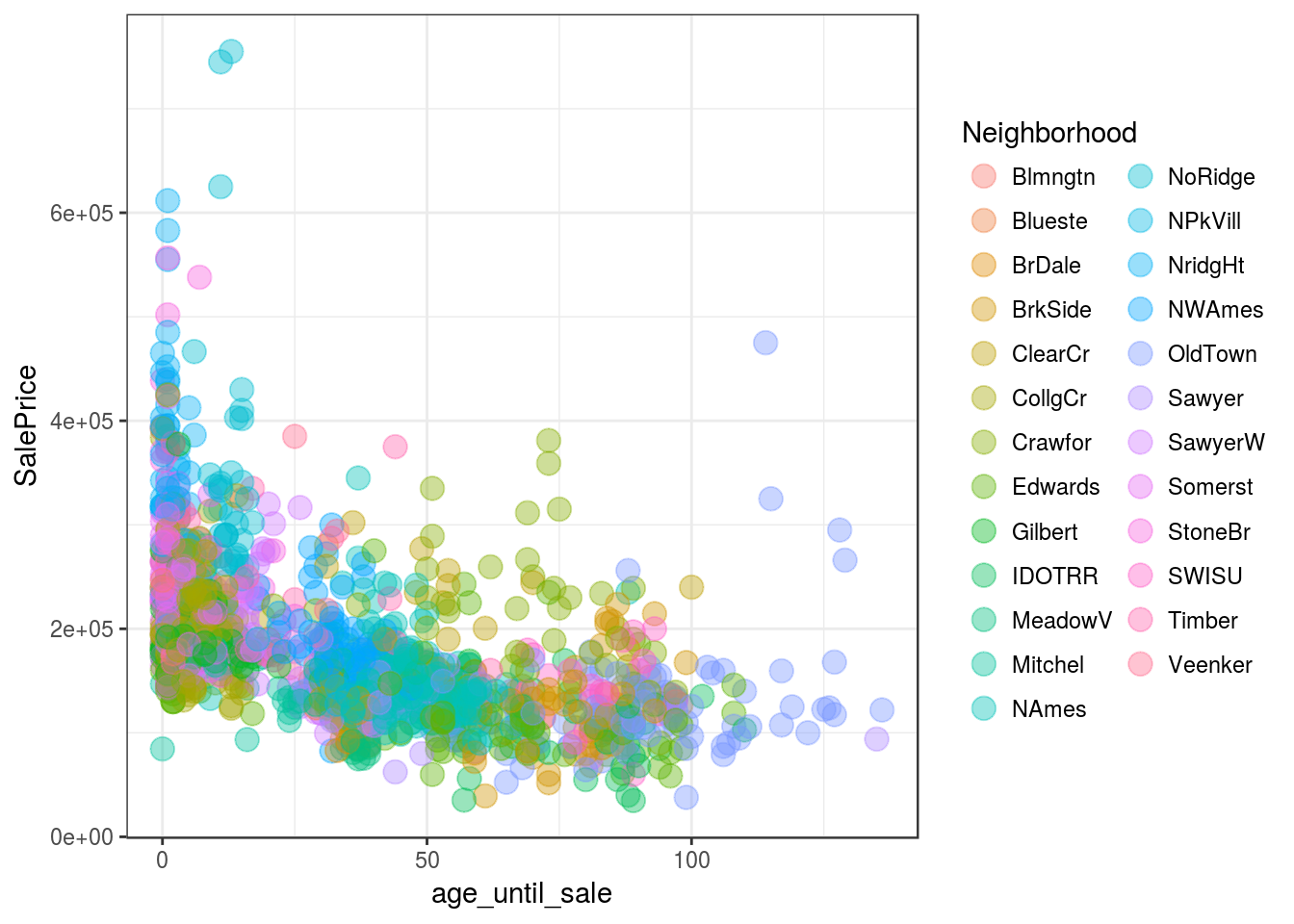
Basement qual tem muita influência no preço da casa.
train %>%
    ggplot(aes(x= BsmtQual, y= SalePrice)) +
    geom_boxplot()+
    theme_bw()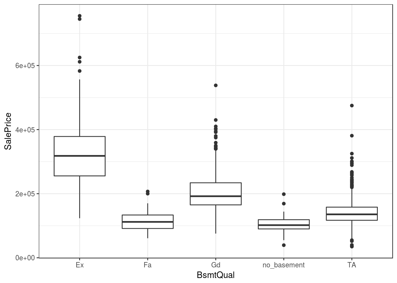
GrLivArea vs SalePrice tem uma relação linear aparente
“Above Grade Living Area Total Sq. Ft. represents the finished above grade living area in a house. It does not include unfinished areas, the area occupied by a cathedral ceiling, enclosed non-living areas such as garages and enclosed porches, or basement area or finished basement living space”.
train %>%
    ggplot(aes(x= GrLivArea, y= SalePrice)) +
    geom_point(size=4, alpha=0.4)+
    theme_bw()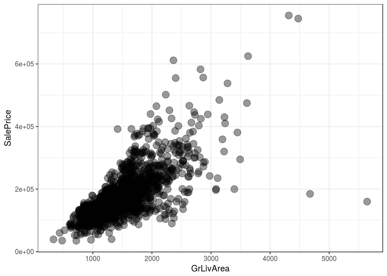
# Fazendo uma regressão com e sem o outlier
summary(lm(SalePrice ~ GrLivArea, data=train))
##
## Call:
## lm(formula = SalePrice ~ GrLivArea, data = train)
##
## Residuals:
## Min 1Q Median 3Q Max
## -462999 -29800 -1124 21957 339832
##
## Coefficients:
## Estimate Std. Error t value Pr(>|t|)
## (Intercept) 18569.026 4480.755 4.144 3.61e-05 ***
## GrLivArea 107.130 2.794 38.348 < 2e-16 ***
## ---
## Signif. codes: 0 '***' 0.001 '**' 0.01 '*' 0.05 '.' 0.1 ' ' 1
##
## Residual standard error: 56070 on 1458 degrees of freedom
## Multiple R-squared: 0.5021, Adjusted R-squared: 0.5018
## F-statistic: 1471 on 1 and 1458 DF, p-value: < 2.2e-16summary(lm(SalePrice ~ GrLivArea, data=train[-which(train$GrLivArea > 4500), ]))##
## Call:
## lm(formula = SalePrice ~ GrLivArea, data = train[-which(train$GrLivArea >
## 4500), ])
##
## Residuals:
## Min 1Q Median 3Q Max
## -197730 -29815 -337 23239 332534
##
## Coefficients:
## Estimate Std. Error t value Pr(>|t|)
## (Intercept) 7168.970 4432.501 1.617 0.106
## GrLivArea 115.040 2.782 41.358 <2e-16 ***
## ---
## Signif. codes: 0 '***' 0.001 '**' 0.01 '*' 0.05 '.' 0.1 ' ' 1
##
## Residual standard error: 53920 on 1456 degrees of freedom
## Multiple R-squared: 0.5402, Adjusted R-squared: 0.5399
## F-statistic: 1710 on 1 and 1456 DF, p-value: < 2.2e-16Interessante: Parece que a area do terreno não influencia muito no preço da casa.
train %>%
    ggplot(aes(x= LotArea, y= SalePrice, col= Neighborhood)) +
    geom_point(size=3, alpha=0.4)+
    theme_bw()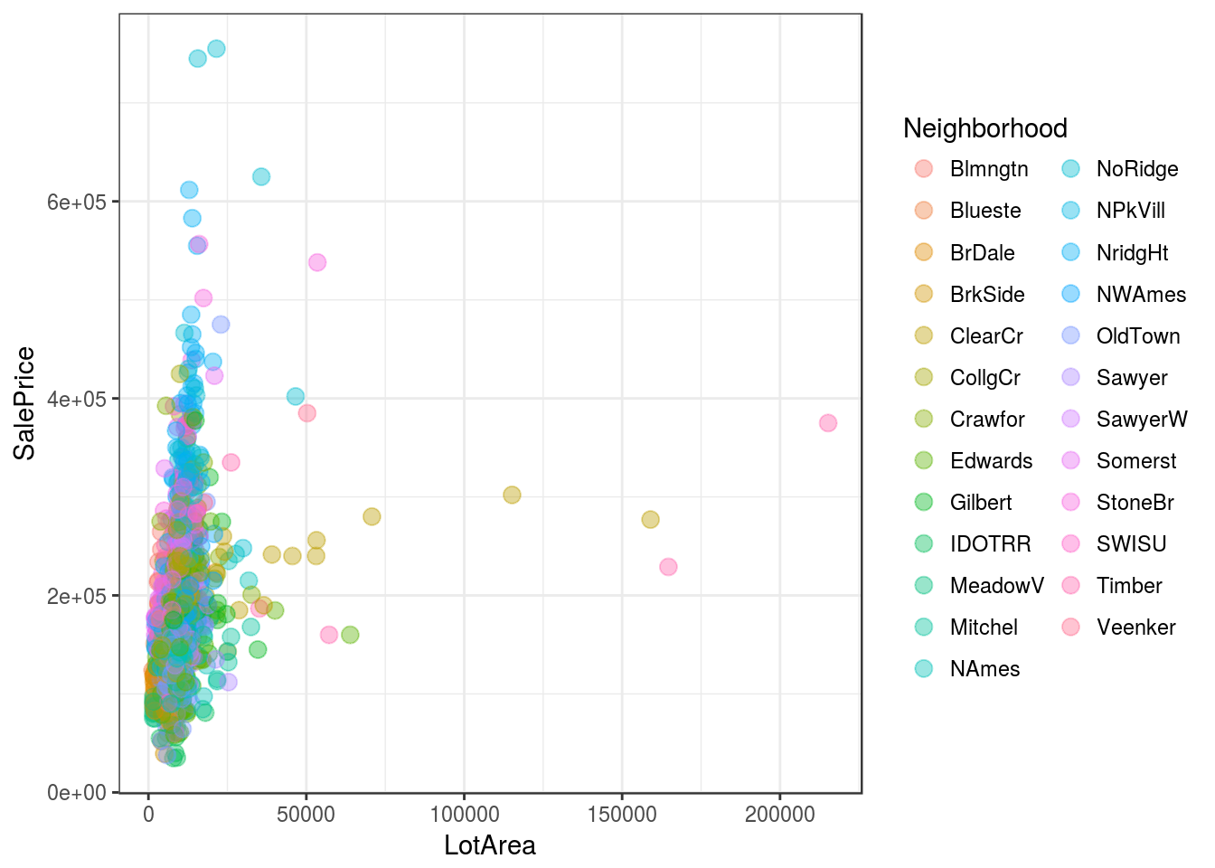
Casas com piscina, sendo elas de boa qualidade, valem muito mais.
train %>%
    ggplot(aes(x= PoolQC, y= SalePrice)) +
    geom_boxplot()+
    theme_bw()
Qualidade da casa vs preço, ótima relação.
train %>%
    ggplot(aes(x= OverallQual, y= SalePrice)) +
    geom_boxplot()+
    theme_bw()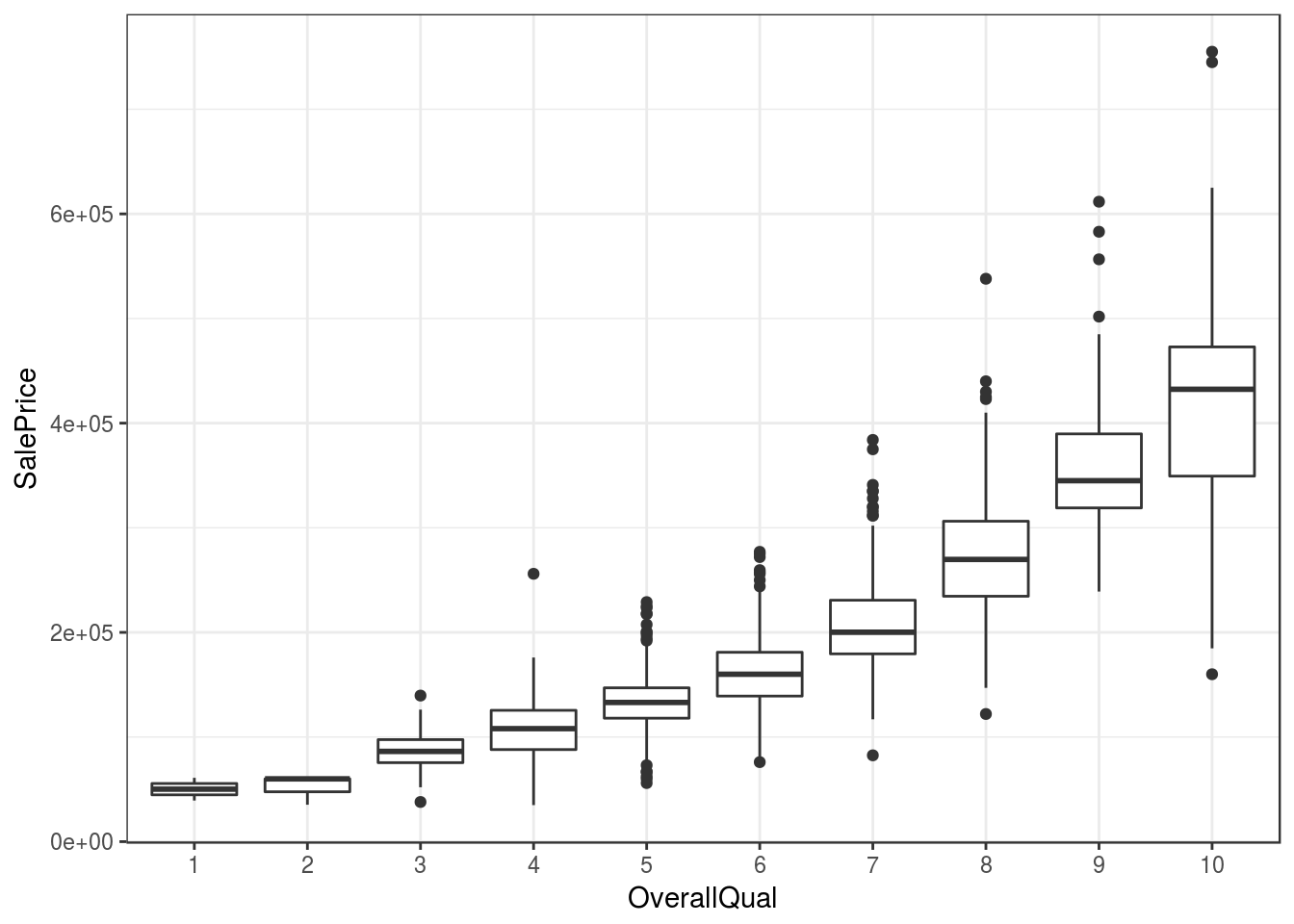
Somei todas as “áreas úteis da casa” para testar se a relação melhora. Ao ver, sim!
train %>%
    ggplot(aes(x= house_useful_area, y= SalePrice, col=OverallQual)) +
    geom_point(size=3, alpha=0.7)+
    theme_bw() +
    scale_color_brewer(palette='Spectral')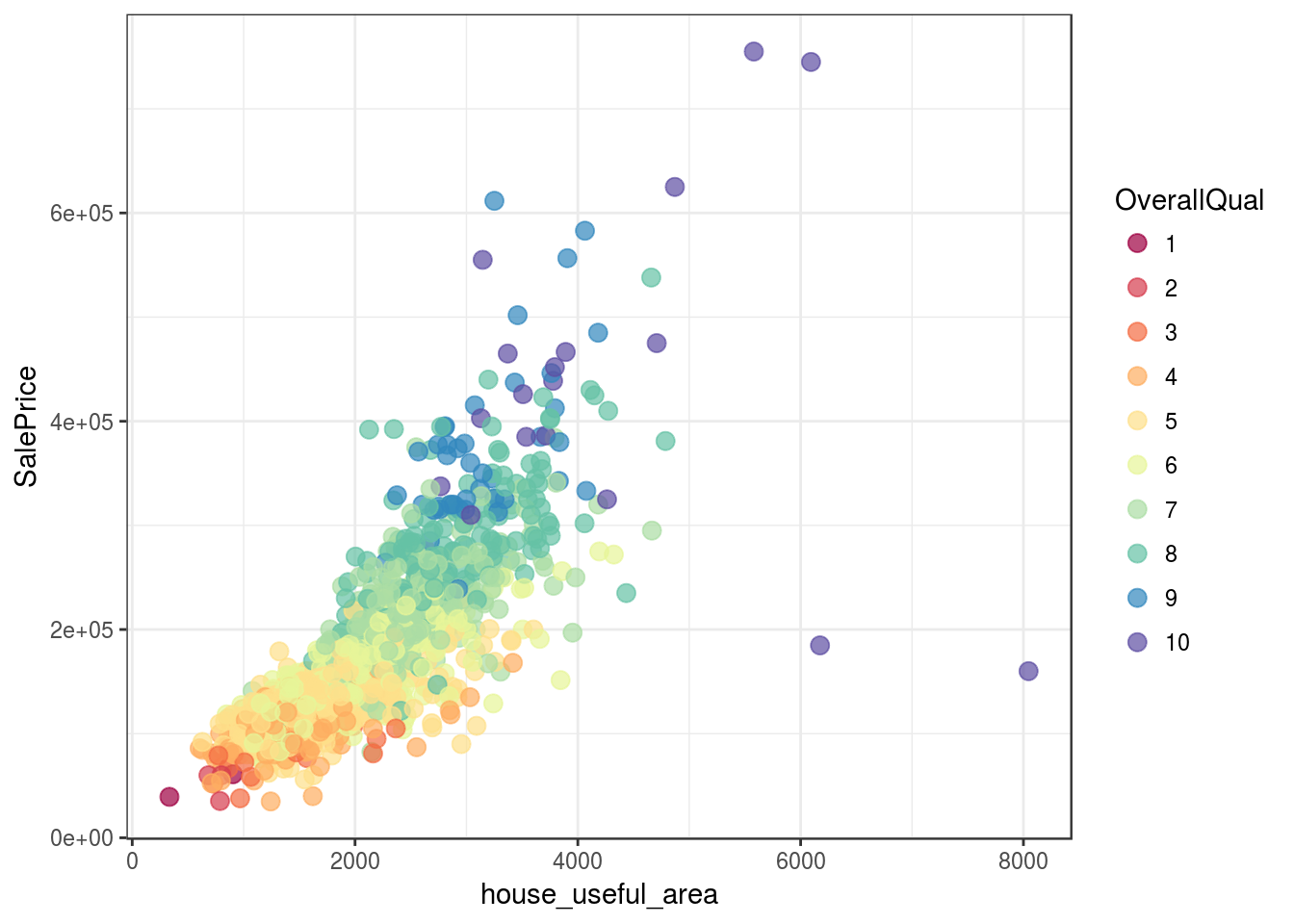
6. Treinando e validando o modelo para o conjunto de teste
6.1. Random forest
random_forest_model <- train(SalePrice~ .,
                             data = train,
                             tuneGrid= data.frame(mtry=c(30, 40, 50, 55, 60,65, 70,75,79,80,82)),
                             method= "rf",
                             trControl= trainControl(method='cv', number=50, verboseIter = TRUE ))
plot(random_forest_model)
print(random_forest_model)

prediction <- predict(random_forest_model, test)
to_submit <-  data.frame(Id= test$Id , SalePrice = prediction)
write.csv(file='prediction_results.csv', to_submit, row.names = F )
6.2.Modelo linear
Testando modelo linear sem os ‘outliers’
lm_model <- lm(SalePrice ~ house_useful_area + OverallQual + GrLivArea +
                   TotalBsmtSF + GarageArea  +
                   ExterQual + X1stFlrSF + BsmtQual +
                   KitchenQual + FullBath +TotRmsAbvGrd,  data=train[c(-524, -1299), ])

summary(lm_model)
summary(train)

prediction <- predict(lm_model, test)
to_submit <-  data.frame(Id= test$Id , SalePrice = prediction)
write.csv(file='prediction_results.csv', to_submit, row.names = F )
summary(to_submit)
6.3.SVM (Support Machine Vector)
svm_model <- train(SalePrice ~ OverallQual + house_useful_area + age_until_sale +  PoolQC + Neighborhood,
      data = train[c(-524, -1299), ],
      method= "svmPoly",
      trControl= trainControl(method='cv', number=3, verboseIter = TRUE ))

plot(svm_model)
print(svm_model)

prediction <- predict(svm_model, test)
to_submit <-  data.frame(Id= test$Id , SalePrice = prediction)

write.csv(file='prediction_results.csv', to_submit, row.names = F )
prediction <- predict(svm_model, train)
6.4.GBM (Gradient Boosting Machine)
metric <- "RMSE"
trainControl <- trainControl(method="cv", number=30)
caretGrid <- expand.grid(interaction.depth= c(1,4,5,6), n.trees= c(2500,3000, 3200, 3400, 3600) ,
                         shrinkage= c(0.1,0.01,0.02,0.03),
                         n.minobsinnode=10)
set.seed(99)
gbm.caret <- train(SalePrice ~ .
                   , data=train
                   , distribution="gaussian"
                   , method="gbm"
                   , trControl=trainControl
                   , verbose=FALSE
                   , tuneGrid=caretGrid
                   , metric=metric
                   , bag.fraction=0.75
)

print(gbm.caret)
plot(gbm.caret)

prediction <- predict(gbm.caret, test)
to_submit <-  data.frame(Id= test$Id , SalePrice = prediction)
write.csv(file='prediction_results.csv', to_submit, row.names = F )
7.1.Resultados obtidos
Ainda há muito a trabalhar nestes dados. O melhor resultado foi obtido com o algoritmo GBM. No Kaggle, conseguimos alcançar uma posição mediana em relação aos demais competidores. Nossa melhor pontuação foi de 0.13477
Posição no ranking geral